python: oxydation des ions iodures par le peroxodisulfate

Enregistrez les noms des espèces et les valeurs des coefficients stœchiométriques dans des variables

nom_A="peroxodisulfate "
nom_B="iodure"
nom_C="diiode"
nom_D="ion sulfate"

coef_A=1
coef_B=2
coef_C=1
coef_D=2

print("le nom de l'espèce A est :",nom_A)
print("le coefficient stoechiométrique de l'espèce A est ",coef_A)

On peut enregistrer ces valeurs de façon plus interactive avec la fonction input()

nom_A=input("nom de l'espèce A ?  ")
nom_B=input("nom de l'espèce B ?  ")
nom_C=input("nom de l'espèce C ?  ")
nom_D=input("nom de l'espèce D ?  ")

coef_A=float(input("coefficient stoechiométrique de A ?  "))
coef_B=float(input("coefficient stoechiométrique de B ?  "))
coef_C=float(input("coefficient stoechiométrique de C ?  "))
coef_D=float(input("coefficient stoechiométrique de D ?  "))

print("le nom de l'espèce A est :",nom_A)
print("le coefficient stoechiométrique de l'espèce A est ",coef_A)

Le milieu réactionnel est constitué d’un mélange de deux solutions aqueuses.5mL de peroxodisulfate à 0.025mol/L et 25mL d’ions iodure à 0.005 mol/L. Déterminez les quantités de matière initiales

VA=5E-3
CA=0.025

VB=25E-3
CB=5E-3

NAi=CA*VA
NBi=CB*VB
NCi=0
NDi=0

print(NAi)
print(NBi)

Calculez xmax et donnez le réactif limitant

nom_A="peroxodisulfate "
nom_B="iodure"
nom_C="diiode"
nom_D="ion sulfate"

coef_A=1
coef_B=2
coef_C=1
coef_D=2

VA=5E-3
CA=0.025
VB=25E-3
CB=5E-3
NAi=CA*VA
NBi=CB*VB
NCi=0
NDi=0

#if(abs(NAi/coef_A-NBi/coef_B)<1E-9):
if(NAi/coef_A == NBi/coef_B):
    xmax=NAi/coef_A
    print("le mélange est stoechiométrique")
elif  (NAi/coef_A>NBi/coef_B):
    print("B est le réactif limitant")
    xmax=NBi/coef_B
else:
    print("A est le réactif limitant")
    xmax=NAi/coef_A
              
print("xmax =  ",xmax)

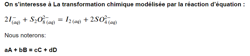
Représentons l’état initial à l’aide d’un histogramme

#py003
import matplotlib.pyplot as plt
nom_A="peroxodisulfate "
nom_B="iodure"
nom_C="diiode"
nom_D="ion sulfate"

coef_A=1
coef_B=2
coef_C=1
coef_D=2

espece= [nom_A, nom_B, nom_C,nom_D]

VA=5E-3
CA=0.025
VB=25E-3
CB=5E-3

NAi=CA*VA
NBi=CB*VB
NCi=0
NDi=0

quantite = [NAi,NBi,NCi,NDi]
bars=plt.bar(espece, quantite,color='grey' )
bars[2].set_facecolor('gold')

plt.grid()
plt.show()

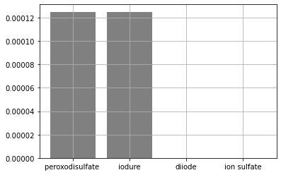
Représentons l’état final à l’aide d’un histogramme

import matplotlib.pyplot as plt
nom_A="peroxodisulfate "
nom_B="iodure"
nom_C="diiode"
nom_D="ion sulfate"

espece= [nom_A, nom_B, nom_C,nom_D]

coef_A=1
coef_B=2
coef_C=1
coef_D=2

VA=5E-3
CA=0.025
VB=25E-3
CB=5E-3

NAi=CA*VA
NBi=CB*VB
NCi=0
NDi=0

xmax =min(NAi/coef_A,NBi/coef_B)

NAf=NAi-coef_A*xmax
NBf=NBi-coef_B*xmax
NCf=NCi+coef_C*xmax
NDf=NDi+coef_D*xmax
quantite = [NAf,NBf,NCf,NDf]

bars=plt.bar(espece, quantite,color='grey' )
bars[2].set_facecolor('gold')
print(xmax)
plt.grid()
plt.show()

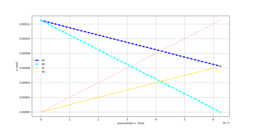
Représentons l’évolution des quantités de matière en fonction de l’avancement.

import matplotlib.pyplot as plt
coef_A=1
coef_B=2
coef_C=1
coef_D=2

VA=5E-3
CA=0.025
VB=25E-3
CB=5E-3

NAi=CA*VA
NBi=CB*VB
NCi=0
NDi=0


x=[]
na=[]
nb=[]
nc=[]
nd=[]

xmax =min(NAi/coef_A,NBi/coef_B)
dx=xmax/50

xi=0
while xi<xmax:
    x.append(xi)
    na.append(NAi-coef_A*xi)
    nb.append(NBi-coef_B*xi)
    nc.append(NCi+coef_C*xi)
    nd.append(NDi+coef_D*xi)
    xi=xi+dx

plt.plot(x,na,'blue',label='nA',marker='o',markersize=5)
plt.plot(x,nb,'cyan',label='nB',marker='o',markersize=5)
plt.plot(x,nc,'gold',label='nC',marker='o',markersize=5)
plt.plot(x,nd,'pink',label='nD',marker='o',markersize=5)

plt.legend()
plt.ylabel('n (mol)')
plt.xlabel('avancement x  (mol)')
plt.grid()

plt.show()

remplaçons les listes par des tableaux numpy

import matplotlib.pyplot as plt
import numpy as np
coef_A=1
coef_B=2
coef_C=1
coef_D=2

VA=5E-3
CA=0.025
VB=25E-3
CB=5E-3

NAi=CA*VA
NBi=CB*VB
NCi=0
NDi=0

xmax =min(NAi/coef_A,NBi/coef_B)
x=np.linspace(0,xmax,50)
na=NAi-coef_A*x
nb=NBi-coef_B*x
nc=NCi+coef_C*x
nd=NDi+coef_D*x

plt.plot(x,na,'blue',label='nA',marker='o',markersize=5)
plt.plot(x,nb,'cyan',label='nB',marker='o',markersize=5)
plt.plot(x,nc,'gold',label='nC',marker='+',markersize=5)
plt.plot(x,nd,'pink',label='nD',marker='+',markersize=5)
plt.legend()
plt.ylabel('n (mol)')
plt.xlabel('avancement x  (mol)')
plt.grid()
plt.show()

Laisser un commentaire Annuler la réponse