livre TS Hatier spécialité physique

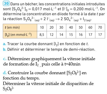
Représentez la concentration en diiode en mmol/L en fonction du temps

import numpy as np
import matplotlib.pyplot as plt
t = np.array([0,10,20,30,40,50,60,70])
C = np.array([0,8.5,12,14,15,16,17,17])

plt.grid()
plt . xlabel ("temps en minute")
plt . ylabel ("[I2] en mmol/L")
plt.scatter(th, C, color='red')
plt.show()

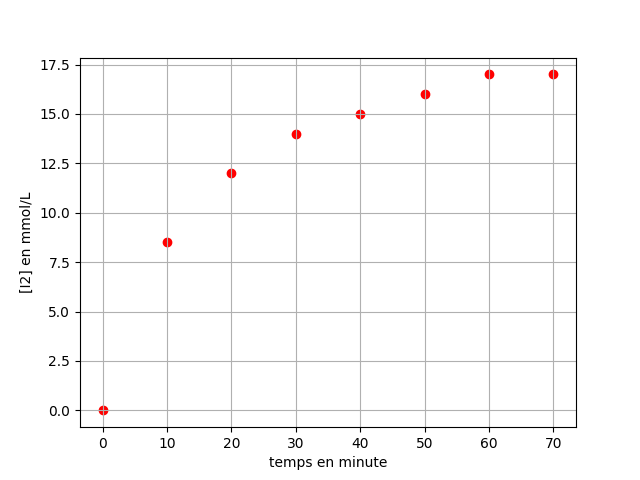
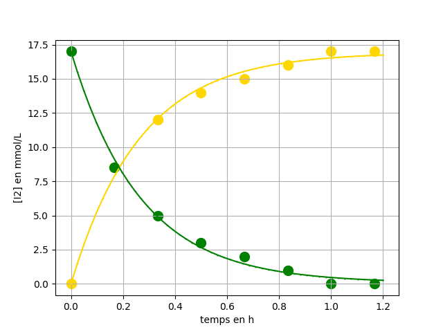
Réalisons un ajustement manuel à l’aide d’un modèle exponentiel en trouvant a et b tels que : [I2]=a*(1-exp(-t/b)) avec t en heure

import matplotlib.pyplot as plt
import numpy as np

t = np.array([0,10,20,30,40,50,60,70])
C_I2 = np.array([0,8.5,12,14,15,16,17,17])
t_h=t/60
t_model=np.linspace(0, 1.2, 50)
def f(t,a,b):
    return a* (1-np.exp(-t/b))

while True:
    c=input("si voulez voulez vous continuer tapez oui?")
    if (c!="oui" ):
        break
    a=float(input( "a ? "))
    b=float(input( "b ? "))
    
    plt.scatter(t_h, C_I2,color="green")       
    plt.plot(t_model, f(t_model,a,b))
    plt.axis([0, 1.2, 0, 20])
    plt.grid()
    plt.show()

Réalisons le même ajustement trouvant a et b tels que : [I2]=a*(1-exp(-t/b)) avec t en heure. modélisation exponentielle avec la librairie scipy (curve_fit)

import matplotlib.pyplot as plt
from pylab import *
import numpy as np
import scipy
from scipy.optimize import curve_fit

t = np.array([0,10,20,30,40,50,60,70])
C_I2 = np.array([0,8.5,12,14,15,16,17,17])
t_h=t/60
t1=np.linspace(0,1.2,50)

coef,cov=scipy.optimize.curve_fit(lambda t,a,b: a*(1-np.exp(-t/b)), t_h, C_I2)

a=coef[0]
b=coef[1]
a=np.round(a,2)
b=np.round(b,2)
print("a= " ,a)
print("b= " ,b)

C1model=a*(1-np.exp(-t1/b))
plt . scatter(t_h ,C_I2,s=100,color ='yellow')
time.sleep(5)
plt . plot (t1 ,C1model,marker=".",color ='blue',markersize=1)
plt . xlabel ("temps en h")
plt . ylabel ("[I2] en mmol/L")
plt . grid ()
plt .show()

Ecrire des lignes de code permettant de trouver le temps de demi-réaction. Convertir dans un second temps ces lignes de code en fonction python.

import numpy as np

t1=np.linspace(0,1.2,50)
C1model=16.92757841*(1-np.exp(-t1/0.26624731))

i=0
while C1model[i]<17/2:
    t_demi=(t1[i]+t1[i+1])/2
    i=i+1
    
print(np.round(t_demi,3),"h")

import numpy as np

t1=np.linspace(0,1.2,50)
C1model=16.92757841*(1-np.exp(-t1/0.26624731))

def temps_demi(t,c):
    i=0
    while c[i]<17/2:
        t_demi=(t[i]+t[i+1])/2
        i=i+1
    print(np.round(t_demi,3),"h")
    
temps_demi(t1,C1model)   

Déterminer les concentration en peroxodisulfate

mauvaise méthode

C_I2 = [0,8.5,12,14,15,16,17,17]

C_S2O8=17-C_I2

print(C_S2O8)

Une solution

import numpy as np
C_I2 = np.array([0,8.5,12,14,15,16,17,17])

C_S2O8=[17-val for val in C_I2]

print(C_S2O8)

Une autre solution

import numpy as np
C_I2 = np.array([0,8.5,12,14,15,16,17,17])

C_S2O8=17-C_I2

print(C_S2O8)

Tracer les deux courbes (diiode et peroxodisulfate) avec les modélisations

import matplotlib.pyplot as plt
import numpy as np
import scipy
from scipy.optimize import curve_fit

t = np.array([0,10,20,30,40,50,60,70])
C_I2 = np.array([0,8.5,12,14,15,16,17,17])

t_h=t/60
t1=np.linspace(0,1.2,50)

coef,cov=scipy.optimize.curve_fit(lambda t,a,b: a*(1-np.exp(-t/b)), t_h, C_I2)
a=coef[0]
b=coef[1]
C1model=a*(1-np.exp(-t1/b))

plt . scatter(t_h ,C_I2,s=100,color ='gold')
plt . plot (t1 ,C1model,marker=".",color ='gold',markersize=1)

C_S2O8=17-C_I2
C2model=17-C1model

plt . scatter(t_h ,C_S2O8,s=100,color ='green')
plt . plot (t1 ,C2model,marker=".",color ='green',markersize=1)

plt . xlabel ("temps en h")
plt . ylabel ("[I2] en mmol/L")
plt . grid ()

plt .show()

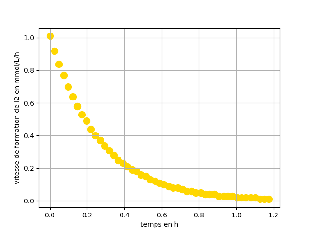
Représenter la vitesse de formation de I2 en fonction du temps. Utilisez le modèle [I2] = 16.927*(1-np.exp(-t1/0.266))

import matplotlib.pyplot as plt
import numpy as np

t1=np.linspace(0,1.2,50)

C1model=16.92757841*(1-np.exp(-t1/0.26624731))

vI2=[]
for i in range (49):
    v=(C1model[i+1]-C1model[i])/(t1[i+1]-t1[i])
    v=np.round(v/60,2)
    vI2.append(v)
    

plt . scatter(t1[:49] ,vI2,s=100,color ='gold')
plt . xlabel ("temps en h")
plt . ylabel ("vitesse de formation de I2 en mmol/L/h")
plt . grid ()

plt .show()